XGSLab Grounding Software and Electromagnetic Analysis Software
SCIENCE FOR ENGINEERING
THE STATE OF THE ART OF THE ELECTROMAGNETIC SIMULATION FOR POWER SYSTEMS, GROUNDING, INTERFERENCE AND LIGHTNING
Electromagnetic Simulation for Power Systems, Grounding, Interference and Lightning
Are you looking for the most advanced and accurate electromagnetic simulation software for power systems, grounding, interference, and lightning analysis?
Look no further than XGSLab. Our software, powered by state-of-the-art algorithms, provides engineers and researchers with the tools they need to design and analyze electromagnetic fields with precision and efficiency. Our user-friendly interface makes it easy to simulate and analyze a wide range of applications, including power systems, grounding, interference and lightning analysis. Optimize your electromagnetic design process and get the results you need with XGSLab, the industry leader in electromagnetic simulation software.
XGSLab stands for eXtended Grounding Software Laboratory.
XGSLab (or shortly XGS) has been chosen by many Universities, Utilities and top Electrical Engineering firms in the whole World.
XGSLab strength points
SCIENTIFIC: based on electromagnetic fields theory and in particular in Maxwell Equations and Sommerfeld Integrals
EASY: a program with an intuitive interface. Very easy even for beginners. Expert users in competitive tools can use XGS right away
OPEN: frequency dependent self and mutual impedances can be exported to EMTP® or ATP® for dynamic behavior studies. Layout data can be imported / exported from / to AutoCAD®. Numerical output can be read by MATLAB®, EXCEL®, and GOOGLE EARTH®
WORLDWIDE: it takes into account International (IEC), USA (IEEE) and European (EN) standards
COMPLETE: a complete virtual laboratory for electromagnetic simulation of Power Systems, Grounding, Interference and Lightning
ADVANCED: based on full-wave PEEC model and suitable for general applications, in a wide frequency range, with arbitrary conductor arrangements and many soil models including multilayer and multizone. Available in the frequency and time domain
POWERFUL: a powerful code that uses parallel computing, advanced math libraries and OpenGL vector graphics
VALIDATED: accuracy validated since 1990 by comparison with analytical cases, published researches, field measures and similar programs
Modules and Applications
XGS includes the modules:
- GSA (Grounding System Analysis)
- GSA_FD (Grounding System Analysis in the Frequency Domain)
- XGSA_FD (Over and Underground System Analysis in the Frequency Domain)
- XGSA_TD (Over and Underground System Analysis in the Time Domain)
- NETS (Network Solver)
- SHIELD (Lightning Shielding)
- SHIELD_A (Lightning Shielding Advanced)
The modules GSA, GSA_FD, XGSA_FD and XGSA_TD are based on the electromagnetic field theory and include the following auxiliary tools:
- SRA (Soil Resistivity Analysis)
- SA (soil resistivity Seasonal Analysis)
- FA (Fourier Analysis direct / inverse) (for XGSA_TD only)
The application field of modules GSA, GSA_FD, XGSA_FD and XGSA_TD is wide because they are based on the PEEC (Partial Element Equivalent Circuit) method, a numerical method for general applications powerful and flexible, a scientific method but perfectly suitable for engineering purposes. This method allows the analysis of complex scenarios including external parameters such as voltages, currents and impedances. The implemented PEEC method solves the Maxwell equations in full wave conditions taking into account the Green functions for propagation, the Sommerfeld integrals for the earth reaction, the Jefimenko equations for electric and magnetic fields and moving from the frequency to the time domain by means the Fourier transforms.
These four modules can import data from “dxf” files, and also export data and results in “dxf” files with a full interactivity with CAD tools. Moreover results can be also exported as “kml or kmz” files and then displayed in Google Earth®.
The module NETS is based on the phase components method and graphs theory and integrates specific routines for the calculation of the parameters of lines, cables and transformers.
The modules SHIELD and SHIELD_A are based on a full 3D geometrical and graphical model and consider the most diffused methods used for the lightning shielding design (Rolling Sphere and Eriksson Methods).
The available calculation options depend on module and license profile. For details on XGS profiles it is advisable to refer to the document “PRICE LIST”.
All modules are integrated in an “all in one” package and provide professional numerical and graphical output useful to investigate any electromagnetic greatness.
All algorithms implemented in XGS are highly efficient in terms of computation speed and have been validated and tested by many Customers in the world.
XGS is easy to use by engineers who need not to be necessarily experts in the specific field, and moreover accurate, stable and fast.
Everything possible has been done to enhance user friendliness and increase productivity to this powerful tool.
GROUNDING SYSTEM ANALYSIS

GSA is a widely utilized and recognized module for grounding and earthing grid calculations and design at low frequency including soil resistivity analysis.
GSA takes into account International (IEC/TS 60479-1:2018), European (EN 50522:2022) and American (IEEE Std 80-2013) Standards.
XGSLab is then also according to widespread national standards or code of practice like for instance Indian (IS 3043:2018) Standards.
GSA is based on a PEEC static numerical model and to the equipotential condition of the electrodes and can analyse the low frequency performance of grounding systems composed by many distinct electrodes of any shape but with a limited size into a uniform or multilayer soil model.
GROUNDING SYSTEM ANALYSIS in the FREQUENCY DOMAIN

GSA_FD is a module for grounding and earthing grid calculation and design in the frequency domain, including soil resistivity analysis and represents the state of the art of advanced grounding software.
GSA_FD is based on a PEEC full wave numerical model and can be applied in general conditions with systems composed by many distinct electrodes of any shape, size and kind of conductor (solid, hollow or stranded and coated or bare) into a uniform, multilayer or multizone soil model in a large frequency range from DC to about 100 MHz. GSA_FD can also consider single core and multicores screened conductors. It is moreover important to consider that GSA_FD is able to takes into account the frequency dependence of soil parameters according to many models and in particular in the model with a general consensus indicates in the CIGRE TB 781 2019.
GSA_FD allows the analysis also of large electrodes whose size is greater than the wavelength of the electromagnetic field as better specified in the following. GSA_FD then overcomes all limits related to the equipotential condition of the electrodes on which GSA is based. With the equipotential condition hypothesis, the maximum touch voltage is widely underestimated and this may result in grounding system oversizing with additional cost sink even 50%.
The implemented model considers both self and mutual impedances. Experience shows that often, mutual impedances cannot be neglected not even at power frequency. A few competitors take into account self impedance and a very few competitors consider the mutual impedance effects and this can lead to significant errors in calculations. Neglecting self impedance effects is often unacceptable, but neglecting mutual impedances can lead to errors over the 20% in calculations also at power frequency. It is important to consider that calculation accuracy often means saving money and indeed, so GSA_FD can allow a significant cost saving in grounding system construction and materials.
GSA_FD can also calculates magnetic fields due to grounding systems or cable, and electromagnetic interference (induced current and potential due to resistive, capacitive and inductive coupling) between grounding systems or cable and pipeline or buried electrodes in general.
In DC conditions, GSA_FD is a good tool for cathodic protection and anode bed analysis with impressed current systems.
OVER AND UNDERGROUND SYSTEM ANALYSIS in the FREQUENCY DOMAIN

XGSA_FD is a module for analysis of aboveground and underground systems in the frequency domain.
XGSA_FD extends the GSA_FD application field to the aboveground systems.
Also XGSA_FD is based on a PEEC full wave numerical model and can be applied in general conditions with same conductors and in the same frequency range of GSA_FD.
Using screened conductors XGSA_FD can simulate gas insulated systems like GIS and GIL.
XGSA_FD can also manage catenary conductors and bundle conductors too and can take into account sources where potential or leakage current and longitudinal current are forced and independent by other conditions. For these reasons XGSA_FD is probably one of the most powerful and multipurpose tool on the market for these kind of calculations.
In addition to GSA_FD, XGSA_FD can calculate electromagnetic fields and interference between aboveground and underground systems (for instance between overhead or underground power lines and installation as pipelines, railways or communications lines).
Moreover XGSA_FD can calculate the electromagnetic force (Lorentz force) on conductors.
Finally, XGSA_FD can consider Surge Protective Devices.
XGSA_FD integrates also some powerful tools for the evaluation of the corona effects (power losses and radiofrequency interference) and the evaluation of the electromagnetic force effects on busbars and supports.
OVER AND UNDERGROUND SYSTEM ANALYSIS in the TIME DOMAIN

XGSA_TD is a module for analysis of aboveground and underground systems in the time domain.
XGSA_TD is a powerful module which extends the XGSA_FD application field to the time domain.
In this regard, XGSA_TD uses the so called “frequency domain approach”. This approach is rigorous and allows considering the frequency dependence of soil parameters.
As known, a transient can be considered as the superposition of many single frequency waveform calculated with the forward Fast Fourier Transforms (FFT).
Using the frequency domain PEEC model implemented in XGSA_FD it is then possible calculate a response for each of these single frequency waveform.
The resulting time domain response can be obtained by applying the Inverse Fast Fourier Transform to all these responses calculated in the frequency domain.
The calculation sequence implemented in XGSA_TD is also called FFT – PEEC – IFFT.
XGSA_TD has been tested for the simulation of transients with a maximum frequency spectrum up to 100 MHz and then can be used for switching transients, lightning and also in fault transients in GIS.
XGSA_TD can consider transients with known equations like Double Exponential, Pulse or Heidler (transients used in EMC studies).
XGSA_TD can also consider transients with arbitrary equations or recorded and then known as a discrete number of samples (transients used in lightning and HV studies).
Moreover XGSA_TD can calculate the electromagnetic force (Lorentz force) on conductors.
XGSA_TD includes an option to export frequency dependent self and mutual impedances to EMTP® or ATP® in order to simulate with a rigorous model the dynamic behaviour of large grounding systems during electromagnetic transients.

LIGHTNING SHIELDING

SHIELD is a powerful full 3D graphical application for the evaluation of the protection of structures from direct lightning strokes using the Rolling Sphere and the Eriksson methods.
SHIELD is based on a numerical model that consider vertical direct lightning strokes, and is then suitable for structures of any height or up to 60 m height in case of relevant protrusions such as balconies or viewer platforms.
SHIELD takes into account International (IEC 62305-3:2012), European (EN 62305-3:2012) and American (IEEE Std 998-2012) Standards but as known, the Rolling Sphere Method is considered by many other standards (NFPA, AS …).
When the Rolling Sphere Method is set, SHIELD first generates a 3D surface corresponding to all possible points that can be touched by the surface of the sphere with a specific radius as it rolls over the air termination system. The air termination system can be composed of any combination of masts and wires (catenary wires included). This surface defines the protected volume.
The protected volume is then superposed to the structure to be protected. The parts of the structure to be protected that protrudes over this surface are not protected.
If the method is applied to the structure to be protected, it can identify the possible lightning strokes impact points and gives indications for the air termination positioning.
When the Eriksson Method is set, SHIELD generates the collection area of air termination system and structure to be protected.
The lightning protection system is effective when collection area of air termination system includes collection area of structure to be protected.
The User can modify the lightning protection system and generate again the protected volume or collection areas. This iterative process allows to get an effective shield.
GROUNDING SYSTEM ANALYSIS

SHIELD_A is a powerful full 3D graphical application for the evaluation of the protection of structures from direct lightning strokes using the Rolling Sphere method.
SHIELD_A is based on analytical model that consider vertical and lateral direct lightning strokes, and is then suitable for special structures of any height and shape.
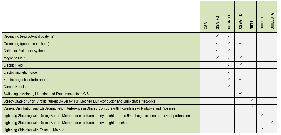
- Product Comparison Chart
- Comparing GSA to GSA_FD
- Comparing XGSA_FD to XGSA_TD
- Uniform, Multilayer and Multizone Soil Models
- The Earth Reaction

The following table summarizes the main assumptions on which GSA and GSA_FD modules are based.
|
Aspcts taken into account |
GSA |
GSA_FD |
|
Resistive coupling |
Yes |
Yes |
|
Capacitive coupling |
No |
Yes |
|
Self Impedance |
No |
Yes |
|
Mutual Impedanc |
No |
Yes |
|
Soil parameters |
ρ |
ρ, ε = f(ω) |
|
Propagation law |
1/r |
e-ϒr/r |
The following diagram represents the application domain of the two modules.
The highlighted central area indicates the usual condition at power frequency.
The diagram has been obtained from a parametric analysis using square well-meshed copper grids energized with a current injected in a corner. The analysed parameters were the grid diagonal “D”, the soil resistivity and the frequency.
In its application dominion as defined by the red solid line, the error made by GSA in the GPR and touch voltages calculation is lower than about 10%.
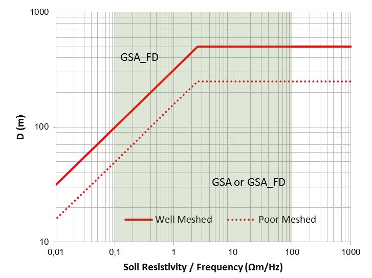
Application domain of GSA and GSA_FD (Log scale)
In practice, in case of well-meshed grids, application limits of GSA can be defined as a function of the wavelength of the electromagnetic field in the earth as follows:
where λ (m) = wavelength, ρ (Ωm) = soil resistivity and f (Hz) = frequency.
The previous diagram indicates that GSA can be used if “D < λ/10”.
This result is in agreement with the simultaneity concept of Albert Einstein.
GSA also requires “D < 500 m” as reasonable limit.
The application limits will be lower if the grid shape is not regular, if the meshes are sparse and if the grid is made of steel or other high resistivity metal. In all these cases, the limit related to poor-meshed grids as defined by the red dashed line should be considered.
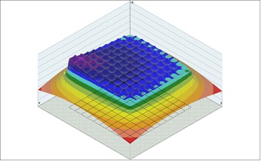
The following three figures show the earth surface potential distribution calculated by applying GSA and GSA_FD to a 100 m x 100 m grid with the same injected current, the same frequency (50 Hz), the same injection point (marked with arrow) and the same soil model.
The qualitative difference between results is evident. GPR and impedance to earth tend to grow whether self impedance and mutual impedance are taken into account. High frequency or low soil resistivity can make this difference even more evident.
Of course, a difference in the earth surface potential distribution corresponds to a difference in touch and step voltage distribution.
In brief, in grounding system analysis at power frequency, GSA can be used in many practical situations but it tends to underestimate the results if the grid size is greater than one tenth of the wavelength of the electromagnetic field, while GSA_FD may be applied in all conditions.
At high frequency, GSA can be applied only to grids with a maximum size of about some tens of meters. In general, at high frequency GSA_FD should be used.
In electromagnetic interference analysis, GSA and GSA_FD can be used respectively for only resistive and resistive + capacitive + inductive coupling evaluation.
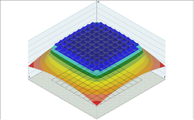
Earth surface potential distribution - GSA (equipotential condition)
Earth surface potential distribution - GSA_FD (only self impedances)
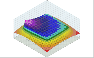
Earth surface potential distribution - GSA_FD (self and mutual impedances)
After these conclusions a question could arise: why not just GSA_FD?
The answer is simple but not trivial.
GSA requires an easier data entry, accept rough layouts, is cheaper and faster than GSA_FD and requires fewer computer resources.
GSA_FD requires additional information about the topology of the conductors system and in order to calculate their self and mutual impedances and a well finished layout.
Moreover GSA_FD requires more experience in the evaluation of results.
If GSA cannot be used, GSA_FD is the right solution.
XGSA_FD is based on the same model of GSA_FD but extended to overhead conductors. The application limits of XGSA_FD can be assumed from DC to about 100 MHz. XGSA_FD greatly expands the application field of XGS and makes it a real laboratory for engineering applications and for research.
XGSA_FD is an irreplaceable tool when conductors are partly overhead and partly underground. This situation is usual in electromagnetic fields evaluation (where sources may be underground cables or overhead wires) or interference analysis (where often the inductor is overhead and the induced is underground).
Anyway XGSA_FD operates to a single frequency.
XGSA_TD can calculate the response in the time domain of a conductors network energized with current or voltage transients.
As known, the methods to calculate the transient behaviour of conductors network in the time domain can be divided into two main categories: those based on the calculation of the solution directly in the time domain and those based on frequency domain calculations and then using the forward and inverse Fourier transforms.
Methods of the first category require low frequency and quasi-static approximations and in addition do not allow considering the frequency dependent characteristics of the grounding system.
Methods of the second category use an electromagnetic field approach for the calculation of the response of the grounding system in a wide range of frequencies and have a good accuracy because they are based strictly on the principles of electromagnetism. On the other hand, in these methods, a system of equations has to be solved for every particular frequency, and a large number of discrete frequency points over the frequency band are chosen to satisfy the frequency sampling theorem.
XGSA_TD is based on the second category methods and uses XGSA_FD as solver in the frequency domain. Then the application limits of XGSA_TD can be assumed as the same of XGSA_FD and in particular the maximum bandwidth of the input transient should be lower than 100 MHz.
This means that XGSA_TD can consider transient input as switching transients, standard lightning currents and also fault transients in GIS.
The simulation of lightning represents the most typical application of XGSA_TD.
The lightning current can be simulated by using the standard short stroke wave form IEC 62305: first positive; first negative; subsequent negative.
With the direct Fourier transform, the time domain input transient is decomposed in the frequency domain.
In the following figures the normalized wave shape of the subsequent negative standard lightning current and their normalized frequency spectrum. The spectrum can be neglected when normalized values are lower than about 10-3 - 10-4. The standard lightning bandwidth is lower than a few MHz also for the fastest lighting, the subsequent negative ones.
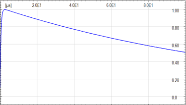
Normalized subsequent negative standard lightning (Linear scale)
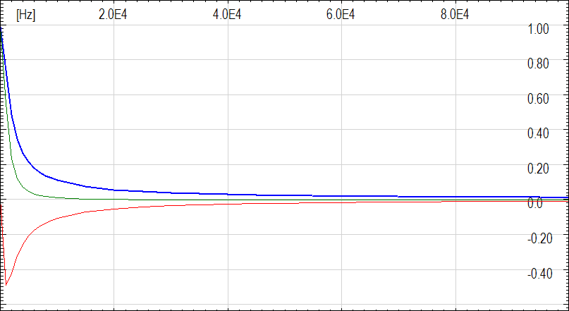
Normalized frequency spectrum – Magnitude, real and imaginary parts (Linear scale)
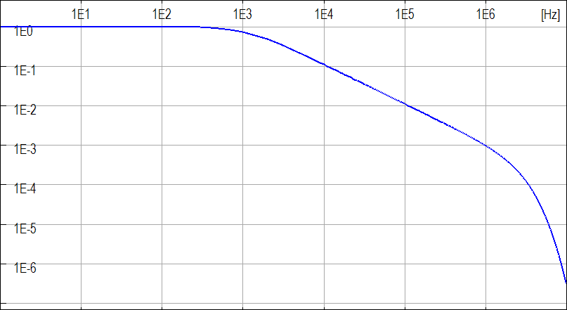
Normalized frequency spectrum – Magnitude (Log scale)
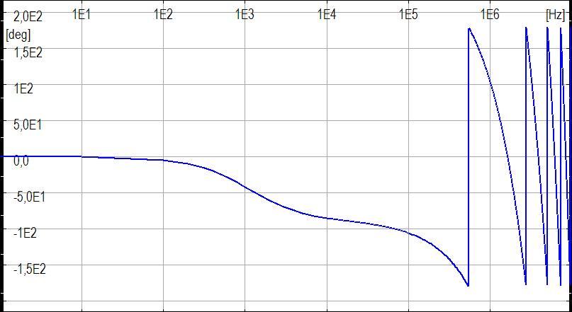
Normalized frequency spectrum – Argument (Log Linear scale)
After the calculation in the frequency domain (taking into account a suitable number of representative frequencies in order to limits the calculation time), the response in the time domain is obtained with interpolation of results and the inverse Fourier transform.
The evaluation of lightning effects is important in many practical applications.
For instance, current generated by a stroke flows in the LPS conductors and dissipate in the soil. The electric and magnetic field generated by such high voltages and currents can cause internal discharges, fires and explosions, may cause damage of equipment and buildings and may be dangerous for people.
In conclusion, XGSA_TD uses XGSA_FD as a calculation engine and Fourier transforms in order to move from time to frequency domain and vice versa.
The choice of the soil model is crucial in electromagnetic simulations of systems close to the soil surface and in particular in the grounding systems analysis. There is much literature about the criteria to set an appropriate soil model which can be used to predict the performances of a grounding system. XGS allows to use uniform, multilayer and multizone soil models.
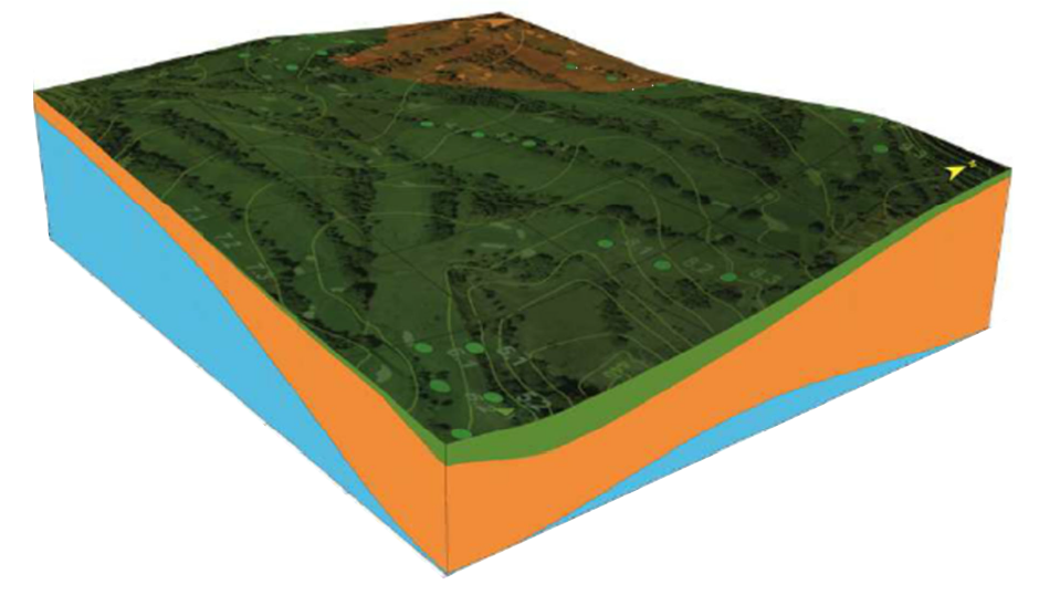
A typical soil cross section including ground water
A uniform soil model should be used only when there is a moderate variation in apparent measured resistivity both in vertical and horizontal direction but, for the majority of the soils, this assumption is not valid. A uniform soil model can also be used at high frequency because in that case, the skin effect limits the penetration depth of the electromagnetic field to a few meters and so, the soil resistivity of the depth layers do not affect the results.
The soil structure in general changes both in vertical and horizontal direction and the presence of ground water further complicates things. The vertical changings are usually predominant on the horizontal ones, but about this aspect, is essential to consider also the grounding system size.
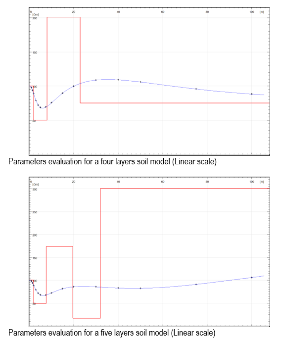
In case of small grounding systems (maximum size up to a few hundred meters), soil model is not significantly affected by horizontal changings in soil resistivity and usually a multilayer soil model is appropriate. The layer number depends on the soil resistivity variations in vertical direction and three, four or five layers can be sufficient for most cases. Sometime, in order to consider seasonal effects on soil model like frozen soil, a bigger layers number can be necessary. For this reason, XGS allows to consider up to 20 layers (limited only in order to avoid unappropriated usage).
In case of grounding systems of intermediate size, soil model is affected by both horizontal and vertical changings in soil resistivity and usually an equivalent double or triple layer soil model is appropriate. This is the most important case in practical applications.
In case of large grounding systems (maximum size over a few kilometres), soil model is significantly affected by horizontal changings in soil resistivity and usually a multizone soil model is appropriate. The zones number depends on the systems size and soil resistivity variations in horizontal direction.
The earth reacts to the AC electromagnetic fields.
The exact solution of this problem was found by Sommerfed and involves integrals (known as Sommerfeld integrals) that represent the solution of the Maxwell equations related to infinitesimal horizontal or vertical current elements radiating in the presence of a lossy half space. Sommerfeld integrals take into account the boundary conditions on the tangential components of the electromagnetic fields at the half space interface.
These integrals usually cannot be solved in closed form and in general are quite difficult to calculate also with a numerical approach because contain very oscillating Bessel functions.
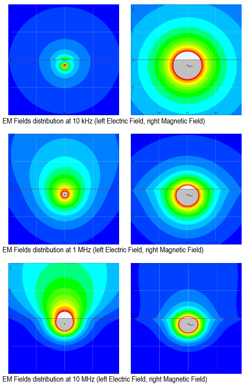
The earth reaction to the AC electromagnetic fields grows with frequency and soil conductivity and is different for horizontal and vertical buried or aerial sources.
In order to display the earth reaction in an effective way, in the following, is represented the cross section of the magnetic field close an horizontal or vertical source on or above the soil surface.
In DC condition, there is no earth reaction.
At low frequency, the earth reaction is negligible for horizontal sources but significant for vertical sources.
At high frequency, the earth reaction becomes always relevant and the earth acts as a mirror for the magnetic field. With vertical sources this happen also at relatively low frequency.
Far from the source, the earth reaction is significant also at low frequency.
The following figures show the electric and magnetic fields distributions related to a single and long overhead line at different frequencies. The calculation area is vertical and across the soil surface.